
IES VisualAnalysis User's Guide
Time History Analysis
The Time History response of a structure is simply the response (motion or force) of the structure evaluated as a function of time including inertial effects. The time history analysis in the advanced level of VisualAnalysis allows four main loading types. These include base accelerations, base displacements, factored forcing functions, and harmonically varying force input.
The harmonic forcing function varies in a sinusoidal fashion and requires Ao and ω to be specified. The equation takes on the form A(t) = Ao*sin(ω*t) and A(t) multiplies all static loads placed in the time history load case at various times. Harmonically varying loads are probably most common when analyzing the effects of machinery on a structure. Often unbalanced rotating machinery or parts are most applicable. Note that the units on ω are such that ω*t has angle units of radians.
The Load Amplitude time history option essentially uses a text file to specify the fraction of the load at specific times. The text file requires two columns, time (t) and A(t) which is the amplification factor. Shown below is a sample of what would appear in the text file along with a plot of the data. Note the text "Force" on the first line. When this text file is read into VisualAnalysis the first line indicates the type of data.
Force
0.0             0.0
0.05            1.0
0.1             1.0
0.1001  0.0
9.0             0.0
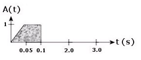
As with the harmonic function, A(t) multiplies the static loads applied to the structure in the time history load case at various times. Load Amplitude loads are commonly used to model wind loads, impact loads, and possibly blast loadings.
Like the Load Amplitude loading type, the Base Displacement uses a text file for input. The base displacement is exactly as it sounds, the structure is forced through some varying ground displacement over time. These displacements can act independently in the global X, Y, and Z directions. The displacements can be any combination of all or some of these directions. (I.e. If you wanted to model an event at a 45 degree angle to the X and Y directions you could specify the necessary components in the X and Y directions respectively.) Units for the text file are always assumed to be seconds and inches. After the file is read in the data will be converted to the current unit system. For example, if one of the displacement values was 6 in it would be read in as 0.5 ft if your current project units were lb-ft. The text file requires at least two columns and can have up to four (refer to the Text File Notes section below for more information). These columns would be the time, t, ux(t), uy(t), and uz(t).
Displacement
0.0     0.0    0.0     0.0
1.0     5.0    0.0     0.0
2.0    -5.0    0.0     0.0
3.0     5.0    0.0     0.0

Note that the line is extrapolated linearly between the t = 2.0s and t = 3.0s values but our time increments limit the displacement to 2.5 seconds. In the example the uy(t) and uz(t) columns are included but have no effect. Note also that if you are working in a plane structure the uz(t) column will always be ignored.
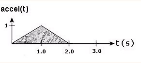
Again, the Base Acceleration loading type uses a text file for input. The base acceleration is very similar to the base displacement and represents putting the structure through some varying ground acceleration over time. Logically, the base acceleration is just the second derivatives of the base displacements. Similarly, the accelerations can act in the x, y, and z directions and again they can be any combination of all or some of these directions. The text file requires at least two columns and can have up to four (refer to the Text File Notes section below for more information). These columns would be time (t), űx(t), űy(t), and űz(t) where the accelerations are specified as a decimal fraction of G (I.e. "0.5" would be 50% of G). Note below the text file is shown in a space delimited format.
Acceleration
0.0   0.0   0.0   0.0
1.0   1.0   0.0   0.0
2.0   0.0   0.0   0.0
2.01  0.0   0.0   0.0
3.0   0.0   0.0   0.0
With the base displacement and base acceleration analysis types static loads only have an inertial effect on the structure. With the harmonic and amplitude analysis types, the static loads applied within the time history case are varied dynamically according to what is specified. For the displacement and acceleration types, VisualAnalysis converts any statically applied load in the time history load case acting in the positive or negative Y direction to a mass. It then has an inertial effect on the results similar to adding lumped mass to nodes. Any statically applied loads that do not act in the gravity direction (positive or negative Y) and any moments are simply ignored by VisualAnalysis and will have no effect on the displacement or acceleration analysis results.
Some general notes about the input text files. The text files can be comma, space, or tab delimited. The Force, Displacement, or Acceleration "headings" on the first line are not essential for the file to work but it is recommended.
Once the data file is opened and read successfully, the data is stored in your project file (*.vap) and the connection to the data file is not maintained. If you edit or modify your data file, you would need to edit the Time History load case to re-load the data from the file. Storing the data file in the project file allows the project to be sent to a colleague or opened at some future time when the text file is not available or may have a different location.
Lastly, the values in the text files are always linearly interpolated until you set a new value. For example, in the sample acceleration data we wanted the acceleration to be zero at a time of 2 seconds and beyond. To accomplish this we specified an acceleration of zero at t = 2.0 sec and also at t = 2.01 sec. If we had not added the t = 2.01 sec entry the program would simply have continued to interpolate a straight line between the acceleration of 1 at t = 1 sec and zero at t = 2.0 sec and continuing on past 2.0 seconds.
In time history analysis procedures there are a number of ways to numerically integrate the fundamental equation of motion. Many of these are discussed in text books including the referenced texts included in this document. VisualAnalysis uses the Newmark method of numerical integration which is considered a generalization of the linear acceleration method. The parameters of the Newmark method are described in what follows.
Number of Steps – This is the number of time steps over which you wish to analyze.
Delta t – This is the time increment for each step. The time step increment can be very important as well. E.L. Wilson in [3] recommends ∆t ≤ 1/(ωMAX*√(γ/2 - β)). For large multi degree of freedom structural systems there is a different limit. This due to computer models of large real structures normally containing a large number of periods which are smaller than the integration time step; therefore, it is essential that one select a numerical integration method that is unconditional for all time steps. For a further discussion refer to [1], [3], and [4].
Gamma and Beta – The Newmark method is basically considered a generalization of the linear acceleration method (Wilson-Theta). Gamma and Beta replaced the 1/2 and 1/6 coefficients on the incremental acceleration terms of the equation for incremental displacement, as derived by the Wilson-theta method. E.L. Wilson presents a good discussion in [3] regarding the beta and gamma parameters for Newmark's method. Many text books on the subject also describe these parameters. The default values of gamma = 1/2 and beta = 1/4 may be used unless you are sure otherwise. These default values make the Newmark method unconditionally stable and provide satisfactory accuracy. Using other values, particularly gamma greater than 1/2 can lead to "numerical damping" and "period elongation".
Delta – Stiffness-proportional damping factor. The Damping Matrix, C, is defined as: C = delta * K. [3]
The unique characteristic of time history cases is you can view results for every time step. A very useful way to look at results is to use the graph feature. For example, while in a Result View you can right click a node in your time history case and select "Graph Node Results" from the context menu. This will allow you to plot displacement, forces, and moments over time for the selected node.
There are three main report items available for time history load cases: Time History Cases, Forcing Function Details, and Forcing Function Summary. The Time History Cases item includes a number of items with the most common ones being the number of time steps, time step increment, gamma, beta, and delta values, and the forcing type. The Forcing Function Details and Forcing Function Summary report items are very similar. They both include the time history case name, the forcing type, the location of the source text file that was used (if applicable) and the number of data points. The only extra information the Forcing Function Details report gives is the data that was read in from the text file in a tabled format. Note that many of the static reports are available at a specific time increment in a time history analysis. For example, you can view member internal forces at any of the time increments during the analysis. Also, the use of enveloped results becomes very useful for processing time history results. Logically, using an envelope would quickly allow you to see the overall maximum and minimum extremes for just the time history case or for multiple load cases. Refer to the Enveloped Results section for more information.