
IES VisualAnalysis User's Guide
Static Analysis
VisualAnalysis supports three methods for static analysis: First Order, P-Delta, and AISC Direct. The Static Method is defined in the Analysis section of the Project Settings settings in the tab.
A first-order analysis is linear and equilibrium is based on undeformed geometry. Since a first-order analysis is linear, the principle of superposition is valid for the analysis results. Often it is best start with a first-order analysis to ensure that a model is stable prior to performing a more advanced second order analysis.
Models that contain one-way members or springs, cable elements, or semi-rigid connections are nonlinear. The principle of superposition is not valid for nonlinear models and should not be used. For nonlinear models, the solution is iterative.
The equilibrium of a deformed bending element that is also subjected to axial force, reveals a nonlinear contribution to the element’s internal moment from the axial force times the displacement (P-Delta).
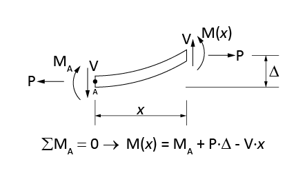
The term “geometric stiffness” is used to describe changes in stiffness due to enforcing equilibrium on the deformed geometry. Structural engineering FEA programs, like VisualAnalysis, typically include geometric stiffness by developing a separate stiffness matrix that is derived from the deformed element’s equilibrium. Including geometric stiffness makes the solution process iterative since internal axial forces are not initially known. However, node positions are not updated during each iteration. Large displacement problems are beyond the scope of this type of analysis.1
When an element is in compression, the geometric stiffness can subtract enough from the linear stiffness that the element becomes unstable. In this situation, the analysis will fail to converge, and the buckled members are identified in the analysis details.
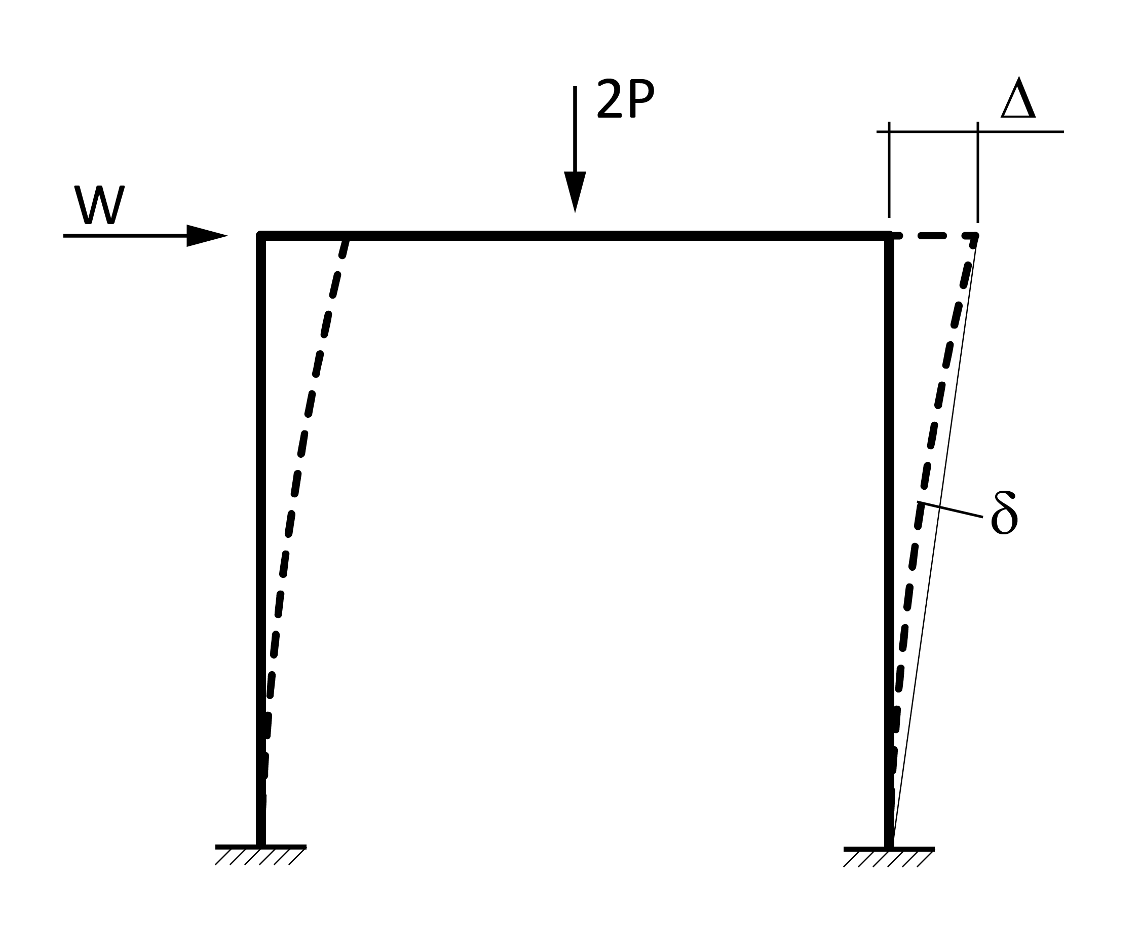
Including geometric stiffness captures P-Δ behavior. To include P-d effects member elements need to be subdivided.
In VisualAnalysis, geometric stiffness can be included for member and plate elements. To include geometric stiffness in the analysis, select P-Delta as the Static Method in the Project Settings. Geometric stiffness is also included in the Direct Analysis Method. The First Order method neglects the interaction between axial load and bending stiffness. Cable elements derive all their flexural stiffness from geometric stiffness, as such geometric stiffness is included for cables regardless of the project’s Static Method.
According to the AISC 360 Specification, the Direct Analysis Method can be used to account for the stability of structural elements and for the structure as a whole. In VisualAnalysis, setting the Static Analysis method to AISC Direct results in a P-Delta analysis (see the previous section), with notional loads and a reduction in member stiffness.
Notional loads are automatically applied to each node of the model. A separate load combination is created for both horizontal directions. These additional load combinations can significantly increase analysis time. The sign of each notional load follows the sign of the load already applied to that degree of freedom. That is, if a node is already being pushed in the positive X direction, the notional load will push it further in that direction. Notional loads are only generated for Strength Level load combinations. While notional loads cannot be viewed in the model directly, their effects can be validated by reviewing the analysis results.
VisualAnalysis automatically reduces the flexural and axial stiffness of member elements as required by the specification. Reductions are a function of the internal axial force in each member. Since these axial forces are not initially known, calculating reductions is an iterative process.
The effective length factor, K, is set to 1.0 for member design when using the Direct Analysis Method. K can be overridden for each design group if desired.
In any situation where a non-linear analysis fails to converge, you can investigate the issue by returning un-converged results (see the project settings). Un-converged results are solutions with reduced loading. While these results are not useful for design, they can help identify an unstable mechanism or the critical load that causes an element to buckle.
The Diaphragm Drift Results report includes the ratio of second order to first order drift in each of the global in-plane directions for each diaphragm level in the structure. The report includes the node and second order drift for the location where the maximum 2nd-Order/1st-Order ratio value is listed.
The Member Moment Magnification table lists the 2nd-Order and 1st-Order moments for each member and the ratio of 2nd-Order/1st-Order moments. The result case where the largest ratio occurred is also indicated in parenthesis, keyed to a Result Cases table that may also be included in the report.
When modeling with Plate Elements it is important to recognize that the results are approximate and a mesh refinement must be performed until the results converge to get an accurate solution. For more information, see the Plate Elements section.